import numpy as np
P = np.array([1.8, 2.1, 2.7, 3.4]) # [mm/d] precipitation
mean_P = np.mean(P)
print(f"Mean precipitation: {mean_P:.1f} mm/d")Mean precipitation: 2.5 mm/dQuarto is a publishing system that lets you write formatted text (Markdown), code (Python, R, Julia) and the output of that code (figures, tables) together in a single document (.qmd). You then render that document to HTML, PDF or Word. This tutorial itself is written in Quarto.
For basic text formatting (headings, bold text, lists, links, …) you use Markdown syntax; the details of which will not be repeated here.
To get started, follow the installations instructions at https://quarto.org/docs/get-started/
A basic intro to on how to use Quarto in VS Code can be found here. The brief summary of the process is as follows:
.qmd file open, run the Quarto: Preview command (Ctrl+Shift+K, or the Preview button top-right of the editor) to render the document and open a live preview next to your source.See Render and Preview for details. Note that VS Code is not the only way to interact with Quarto documents, as you can for example also use it from RStudio.
If you have problems with running the preview via the button or Ctrl+Shift+k command in VS Code, you can also manually launch it via the terminal:
quarto preview --no-browser, which returns output similar to (xxxx is used to denote the port number, which may vary):Preparing to preview
Watching files for changes
Browse at http://localhost:xxxx/
Listening on http://127.0.0.1:xxxx/http://localhost:xxxx/ to open the preview in VS Code.A code block (chunk) starts and ends with three backticks, with {python} right after the opening backticks. Extra chunk options go on separate lines starting with #|, right at the top of the chunk. Type this yourself in a .qmd file:
```{python}
#| echo: true
import numpy as np

P = np.array([1.8, 2.1, 2.7, 3.4])  # [mm/d] precipitation
print(f"Mean precipitation: {np.mean(P):.1f} mm/d")
```
See the execution options documentation for all available chunk options. An important option is echo: if set to true, the code will be displayed in the the rendered document. So for the chunk above, with echo set to true, so the rendered results looks like:
import numpy as np

P = np.array([1.8, 2.1, 2.7, 3.4])  # [mm/d] precipitation
mean_P = np.mean(P)
print(f"Mean precipitation: {mean_P:.1f} mm/d")
Mean precipitation: 2.5 mm/dIf you set echo to false, the code will not be displayed, but the output of the chunk (here the print statement) will:
Mean precipitation: 2.5 mm/dBefore trying this yourself, make sure you have installed Python via Conda and configured it correctly, as outlined in the Python and VS Code tutorial. For more general info on how to use Python in Quarto, see the Python Quarto documentation.
Additionally, it can also be useful to include variables from your Python code blocks in your text. For example, to include the numeric output of mean_P in your text, you can do so by adding {python} f"{mean_P}", where we use the so-called f-string syntax. This will then render as 2.5.
All details on figures are in the documentation; labelling and referencing is explained under cross-references.
Insert an existing image with Markdown syntax. For a label (needed to reference it) and a caption, use:
{#fig-cat}Rendered, this gives Figure 1:

For a figure produced by Python code, set the label and caption as chunk options label (must start with fig-) and fig-cap:
```{python}
#| label: fig-precipitation
#| fig-cap: "Precipitation over time."
import matplotlib.pyplot as plt

plt.plot(P)
plt.xlabel("Time (days)")
plt.ylabel("Precipitation [mm/d]")
```
Rendered, this produces Figure 2:
import matplotlib.pyplot as plt

plt.plot(P)
plt.xlabel("Time (days)")
plt.ylabel("Precipitation [mm/d]")
plt.show()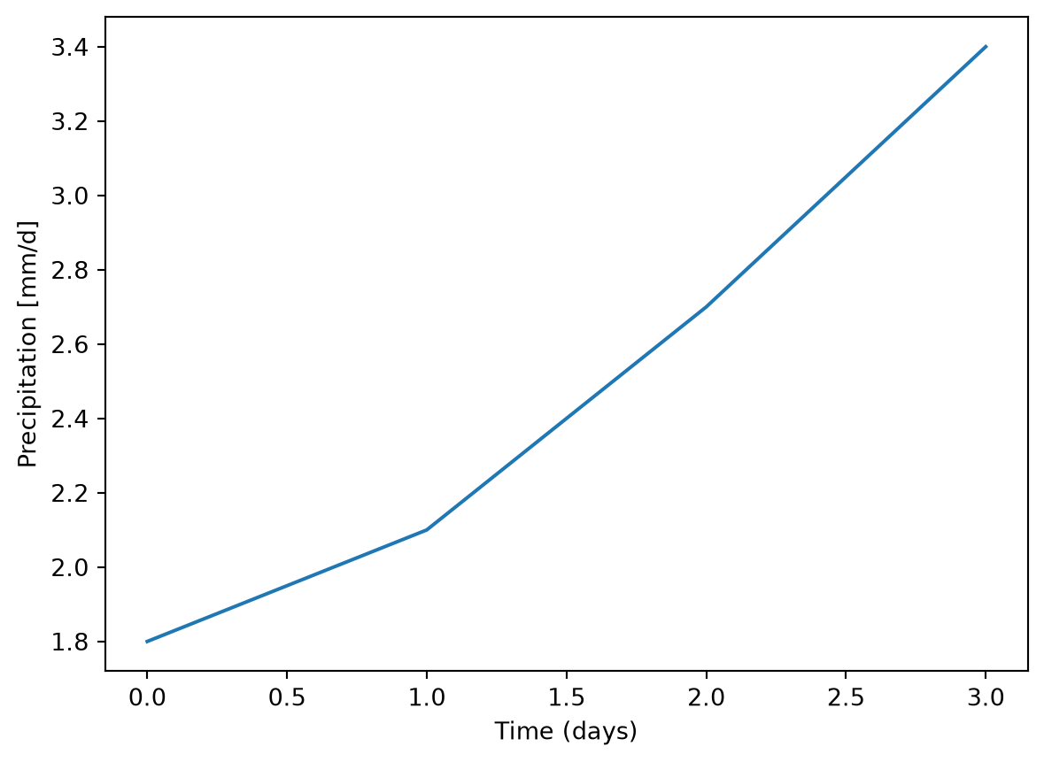
Reference a labelled figure anywhere in your text with @fig-label, e.g. @fig-precipitation gives Figure 2.
All details on tables are in the Quarto documentation; labelling and referencing is explained under cross-references.
Type a table directly in Markdown. Add a label (must start with tbl-) and caption on the line right after the table, preceded by a ::
| Variable | Unit |
|----------|------|
| P        | mm/d |
| Q        | mm/d |

: Overview of the variables used {#tbl-variables}
Rendered, this gives Table 1:
| Variable | Unit |
|---|---|
| P | mm/d |
| Q | mm/d |
For a table produced by Python code (e.g. a pandas.DataFrame), again use the chunk options label (starting with tbl-) and tbl-cap:
```{python}
#| label: tbl-summary
#| tbl-cap: "Summary of the precipitation data."
import pandas as pd

pd.DataFrame({"Mean": [np.mean(P)], "Sum": [np.sum(P)]})
```
Rendered, this produces Table 2:
import pandas as pd

pd.DataFrame({"Mean": [np.mean(P)], "Sum": [np.sum(P)]})| Mean | Sum | |
|---|---|---|
| 0 | 2.5 | 10.0 |
Reference a labelled table with @tbl-label, e.g. @tbl-summary gives Table 2.
As mentioned in Section 1, your Quarto document can be rendered to different output formats. The default is HTML (aka web page format), which works out of the box with Quarto installed.
For PDF output, you need to have a LaTeX distribution installed on your computer. The easiest (and recommended) way do this is is to install TinyTeX by opening the command line and typing:
quarto install tinytexYou can subsequently check if the installation was successful by typing:
quarto toolsYou should see a version (e.g. v2026.09) mentioned under Installed for TinyTex. For more info on PDF output in Quarto, see the documentation.