2 Practical information
Before diving into the exercises, some practical information is provided on how to effectively set up your working environment.
2.1 The repository
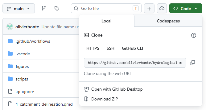
All code used to create this assignment is available at https://github.com/olivierbonte/hydrological-modelling. This collection of files is called a repository. To get started, go the the URL above, click on the green Code button and select Download ZIP (see Figure 2.1). Unzip the downloaded file and place the resulting folder at a location of your choice. This folder contains all the files you need to complete the exercises.
Note that only the code, but also the processed data is now downloaded. You can find this data in data/processed. More info on the data sources and processing is given in Chapter 3.
This assignment is provided to you in two formats, up to you which one you prefer to work with:
- A website at https://olivierbonte.github.io/hydrological-modelling-public/
- A PDF document, which you can download from https://olivierbonte.github.io/hydrological-modelling-public/Exercises-Hydrological-Modelling.pdf
2.2 Working with Quarto and Python
A general introduction to Quarto and Python is given in… LINK TO DEPARTMENT WIDE INTRO HERE LATER.
The idea of this exercise set is that you will use Quarto to combine your code and your scientific report in a single document. The goal is to write a report following the principles of reproducible research1, where others have access to all the data and code needed to obtain the same results as the one you present.
In these practicals, you will therefore not write a report from scratch (in Microsoft Word, Google Docs…), but instead you’ll extend the provided .qmd files for each exercise. The files of interested are numbered from 1_...qmd to 6_...qmd. Here you can add Python code2 for your figures and write your discussion in Markdown.
Don’t perform al your computations inside of the .qmd files! Instead, make a regular .py file inside of the scripts folder for each exercise. From these .py files, you can save the results (e.g. metrics, output data) in (for example) a data/solutions folder. From this folder, you can then import the necessary results in the .qmd files to write your report and make your figures.
2.3 Evaluation
Hand in your report of this assignment via Ufora by ADD DATE LATER. Please hand in:
- A PDF version of your report, which is rendered via Quarto.
- The full set of files (i.e. repository) including your solution as a
.zipfile.
Your report should we written scientifically and should contain at least the following:
- A summary of the results with reference to relevant figures and metrics, and a proper discussion. Note that all tasks are related and that the results should be discussed in reference to one another in a scientific manner. The emphasis of the report should be on this part. This part should be used to draw the attention on shortcomings of the different algorithms and make a link to potential alternatives. Use the sections
Results and discussionin1...qmdto5...qmdfor writing this part down. - A conclusion about the modelling exercise as a whole, which is written in the
6_conclusion.qmdfile. - To support your discussion, it is valuable to include references to relevant scientific papers. To add a reference, please include the relevant source in its bibxtex format to
references.bib. More information on how to handle citations in Quarto can be found here. The bibtex format is explained in this guide. By means of example, one scientific article, Moore (2007), is already included.
This concept is introduced in your course on Data Science in the 2nd Bachelor year of Bioscience Engineering, where you made a Quarto/Rmarkdown presentation/report for a data analysis↩︎
As an example of how this is used in practice, see e.g. the source file
0_study_area_and_data.qmdfor Chapter 3↩︎